Impacts of abrupt land cover changes on French common birds

Table of Contents

1. Data
   1. Temporal Monitoring of Common Birds | STOC
   2. Annual land cover products | GLC_FCS30D
   3. Intersection | STOC ∩ GLC_FCS30D
2. Objectives
3. Detection of abrupt landscape changes
   1. NaviDAM for detection
   2. Hands-on outlier detection
   3. Detection events aligned on bird abundance curves
4. Bird diversity metric shifts attribution
   1. NaviDAM for attribution
   2. Hands-on synthetic controls
   3. Perspectives
5. References

Biospace25 presentation introducing the study context and first results available on HAL.

Observed biodiversity changes can be hard to attribute to their pressures since they are often highly entangled and barely measured.

In this Gallery page, we showcase how NaviDAM can be used to guide method selection (with the filtering motor) after introducing the data & objectives.

Data

Temporal Monitoring of Common Birds | STOC

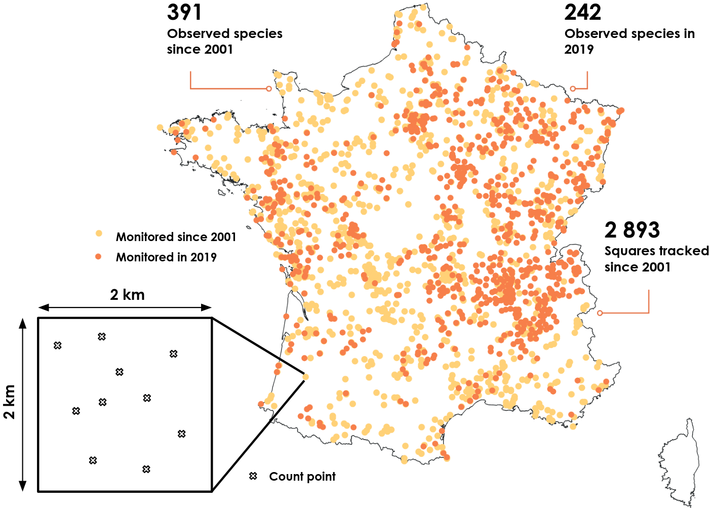
STOC is a standardized count protocol of common birds in France, with data available on the study period 2001-2019 (protocol change in 2001). Partipant observers focus on 2x2 km squares monitored according to an annual random draw, see Figure 1.

Figure 1: STOC coverage in mainland France. Source: (missing reference)

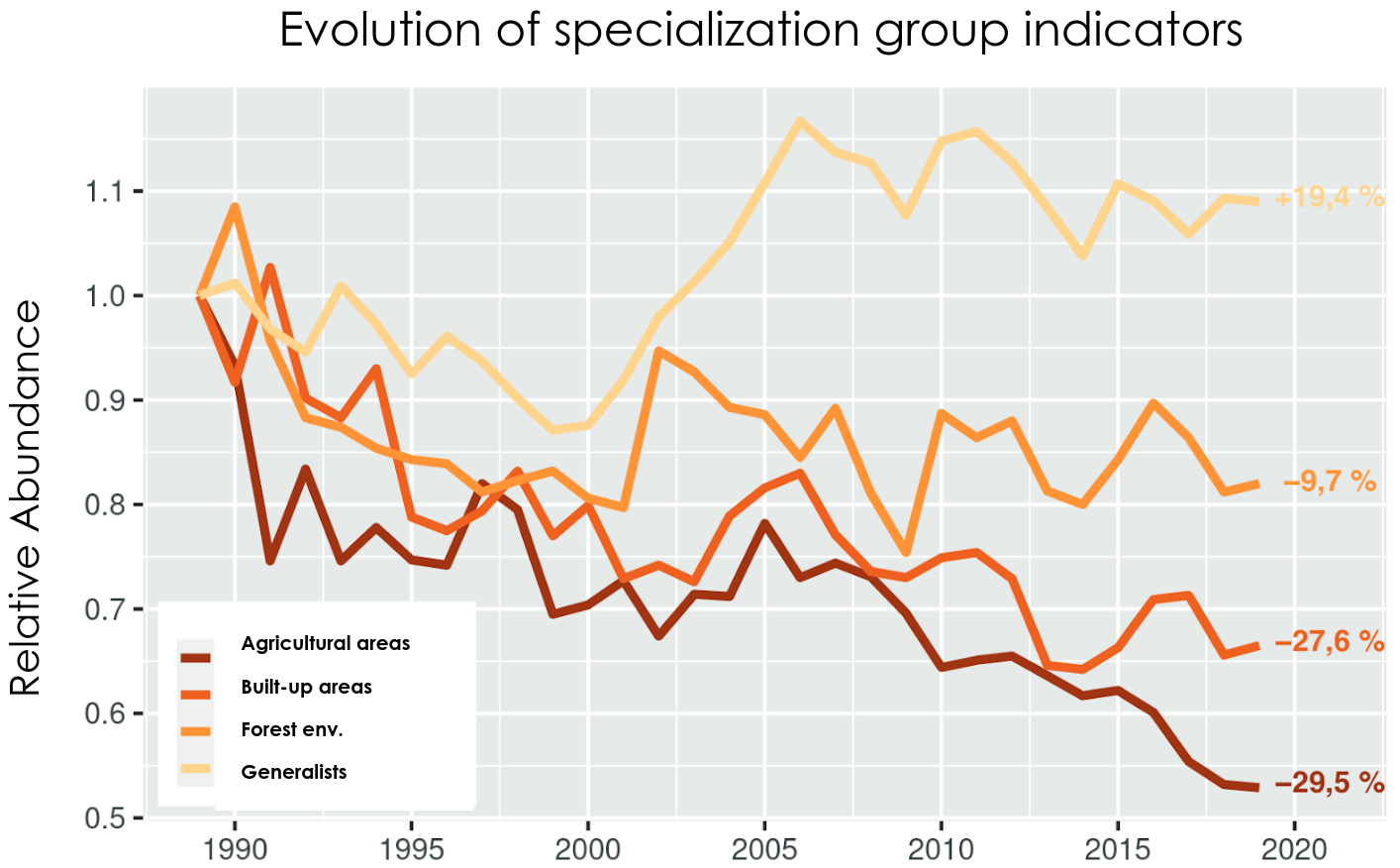
This survey enables studying the evolution of specialization groups of birds through time:

Figure 2: 75 species are used to construct indicators based on their specialized habitats. Source: (missing reference)

Example abundance curves per observation plot

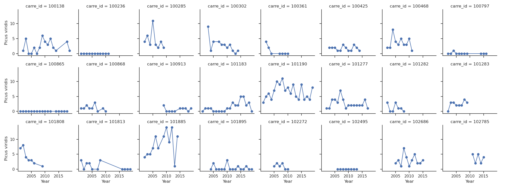
On Figure 3 we plot the monitored abundance of one common species, Picus viridis, for a selection of observation squares to give a sense of sampling effort.

Figure 3: Picus viridis abundance for a selection of observation squares.

Abundances can also be summed by bird specialization group like in Figure 4, but still appreciated by observation square: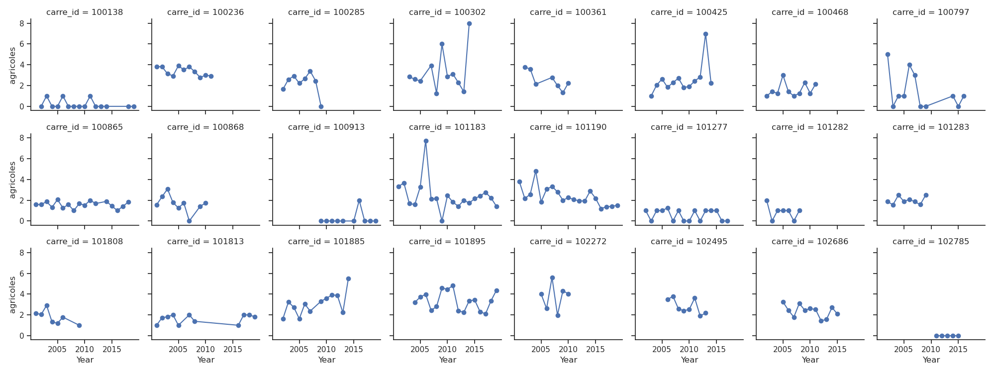

Figure 4: Abundance of bird species specialized in agricultural areas for a selection of observation squares.

It is on this type of bird abundance curves that we will test later in the attribution section if the detected land cover changes (see hands-on detection) have an impact.

Annual land cover products | GLC_FCS30D

The annual land cover data products originate from Zhang et al. (2024). It has a 30-meter resolution as based on Landsat imagery, 35 land-cover categoties spanning from 1985 to 2022 (every 5 years before 2000, annual after), see Figure 5. The tiles were downloaded from the project’s Zenodo and merged as annual mosaics over France using GDAL command lines.

Figure 5: The overview of the GLC_FCS30D dataset during 1985 to 2022. Source: Liu, Zhang, & Zhao (2023)

Intersection | STOC ∩ GLC_FCS30D

We extracted land cover data on the 2x2-km squares matching the STOC survey squares, see the example STOC squares on Figure 6. It results in short time-series as illustrated Figure 7.

Figure 6: Example STOC observation squares used to intersect the land cover products.

Figure 7: Example land cover time-series of STOC observation squares. Open in maps: 1. 2. 3. 4.

Objectives

The objective of this work is twofold:

1. Detection To identify STOC monitoring squares that have been affected by abrupt landscape changes. To achieve this, we first compute landscape metrics on the annual land cover squares, and second look for a suited detection method with NaviDAM.
2. Effect estimation To test if the detected landscape changes result in bird diversity metric shifts. If we succeed in estimating significant effects, we could therefore confidently attribute or not the diversity shifts to the land cover changes.

Detection of abrupt landscape changes

• Using PyLandStats (Bosch, 2019), we computed landscape metrics on the successive land cover annual squares as depicted Figure 7. For the list of available metrics, see PylandStats publication’s Table S1. We also relied on their user-friendly notebooks for easy implementation. The R equivalent package is landscapemetrics.

• Then, we tested several landscape metrics assumed to be ecologically relevant for bird populations (e.g. according to the forest edge effect): ["proportion_of_landscape", "number_of_patches", "largest_patch_index", "total_edge", "landscape_shape_index", "contagion", "shannon_diversity_index"].

The objective now is to find a suitable detection method for identifying abrupt changes in landscape metrics. To achieve this, we can use the NaviDAM tool.

NaviDAM for detection

On the home page, we reach the User input invite to evaluate the task needs:

• We start by choosing the objective Detection:

Figure 8: Detection user input | Objective and data options.

• And now describe our data:
  • Type: We have Panel data, i.e. time-series for different samples (here the STOC observation squares).
  • Time-series length: We have 26 time steps, so ≥ 10 and < 100.
  • Handles few samples: No need, we have thousands of points.
  • Scalable to big data: No need idem. Even if we scale up the study to other monitoring programs, the relative scarcity of standardized data doesn’t require big data approaches.
  • Handles missing data: Simple corrections feasible even if we have complete time-series here, we prefer imposing this condition in case remote sensing data would be missing when upscaling the study.
  • RS-data proven: At least few RS applications exist no special need to rely on a estbalished method with RS data (land cover here), few applications would be enough.

 

Figure 9: Detection user input | Model properties.

• Next, the desired model properties (criteria have been adapted to the Detection objective):
  • Requires explicit processes: Agnostic No knowledge nor a priori on the expected change form apart than being abrupt.
  • Exposure type: Binary Monitoring abrupt land cover changes implies having a Before/After study design.
  • Number of variables: Univariate Even if we test various landscape metrics, we consider them one after the other.

 

Figure 10: Detection user input | Packages.

• About the packages, simple expectations :
  • Language: Python, R We prefer here these two common programming languages for running analyses in batch.
  • Usage: User-friendly, Technical but well documented To keep analyses easily reproducible.

 

Figure 11: Detection user input | Assumptions.

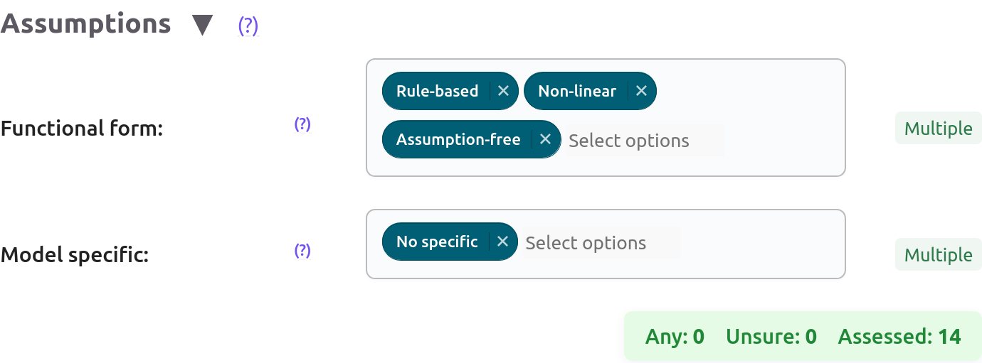
• Finally the assumptions, again adapted to the Detection objective:
  • Functional form: Rule-based, Non-linear, Assumption-free Expecting an abrupt change to be detected, the best option is likely Rule-based with a rule level fitted on the data. However, we also keep other options to avoid being too stringent on the method sub-selection & retain more candidate methods.
  • Model specific: No specific No particular expectation.

--> All criteria have been assessed so the counter on the right turns to green.

 

Figure 12: Detection user input | Result.

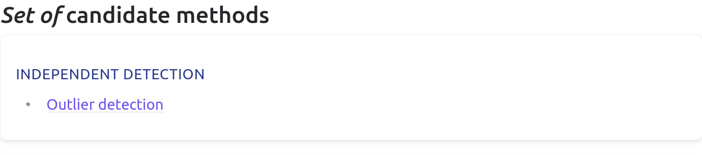
Status

For now, only the method family Outlier detection matches the specified criteria and the page hasn’t been documented yet. To speed up NaviDAM implementation, see the contributing page. However, this case study page already illustrates how the filtering tool can be used to find candidate methods suited to your project.

Eventually, different methods will be suggested after such an exercise, and users will then be able to consult the corresponding documentation pages and jump to the relevant resources to inform their method choice.

Hands-on outlier detection

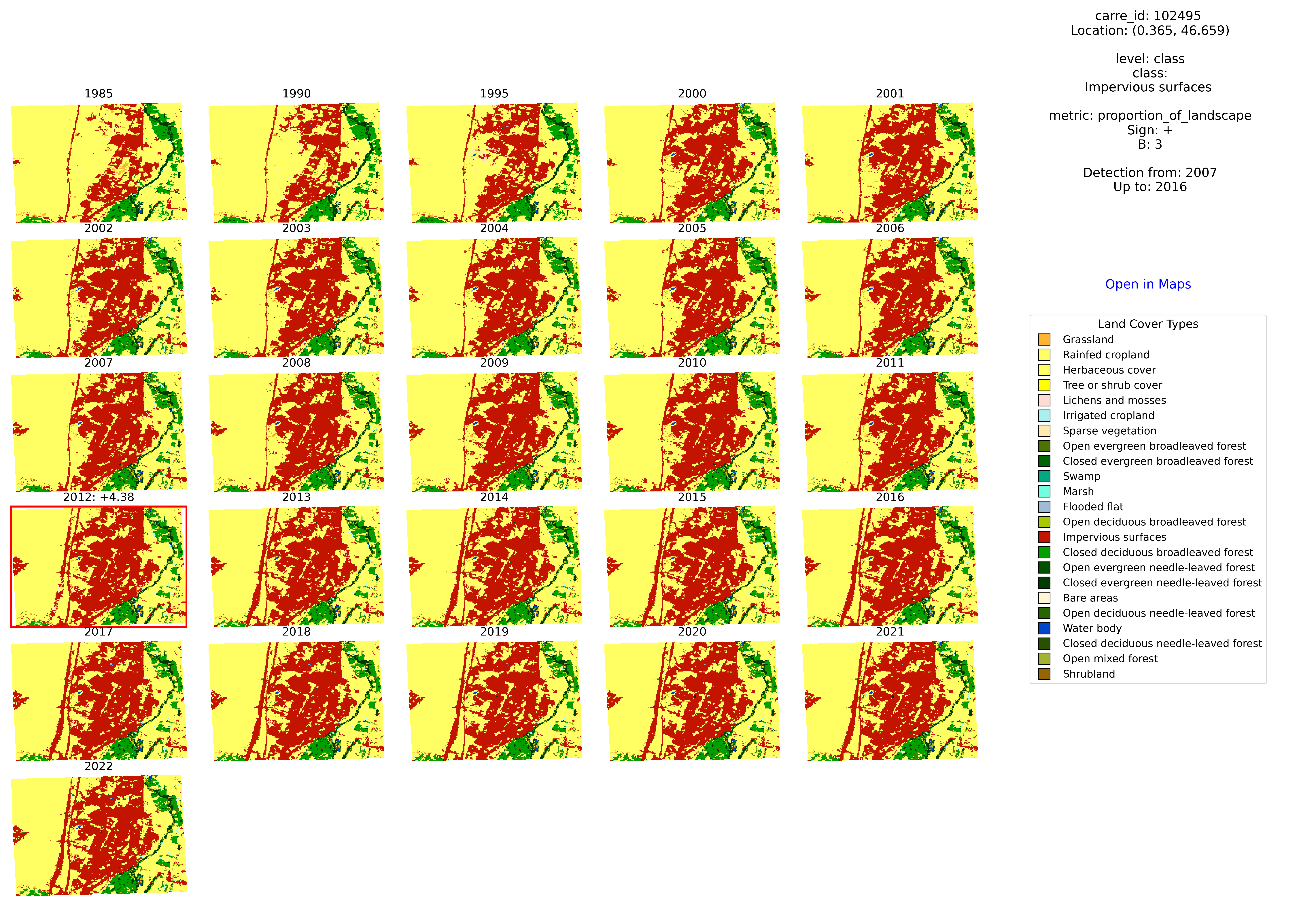
Abrupt changes were defined as a deviation superior to B standard deviation to the average annual change. It allowed detecting plots affected by sudden landscape change and at which years.

Outlier detection as extreme deviation from mean annual change

In this case study, we simply detected abrupt changes by:

• Choosing a target level: landscape / class metrics
  • If class, choosing a target class, e.g. Impervious surfaces
• Choosing a target metric and sign, e.g. proportion_of_landscape / +
• Choosing a deviation level with B, see this table for corresponding proportions.
• Then, we compute the interval I of time-series within the tolerated deviation range for the chosen metric as: I = [avg - B*std, avg + B*std] after standardizing the successive annual changes.
• Finally, we identify the time series affected by extreme land cover changes that i) ∉ I, and ii) are either positive, negative or both depending on the chosen sign.

 

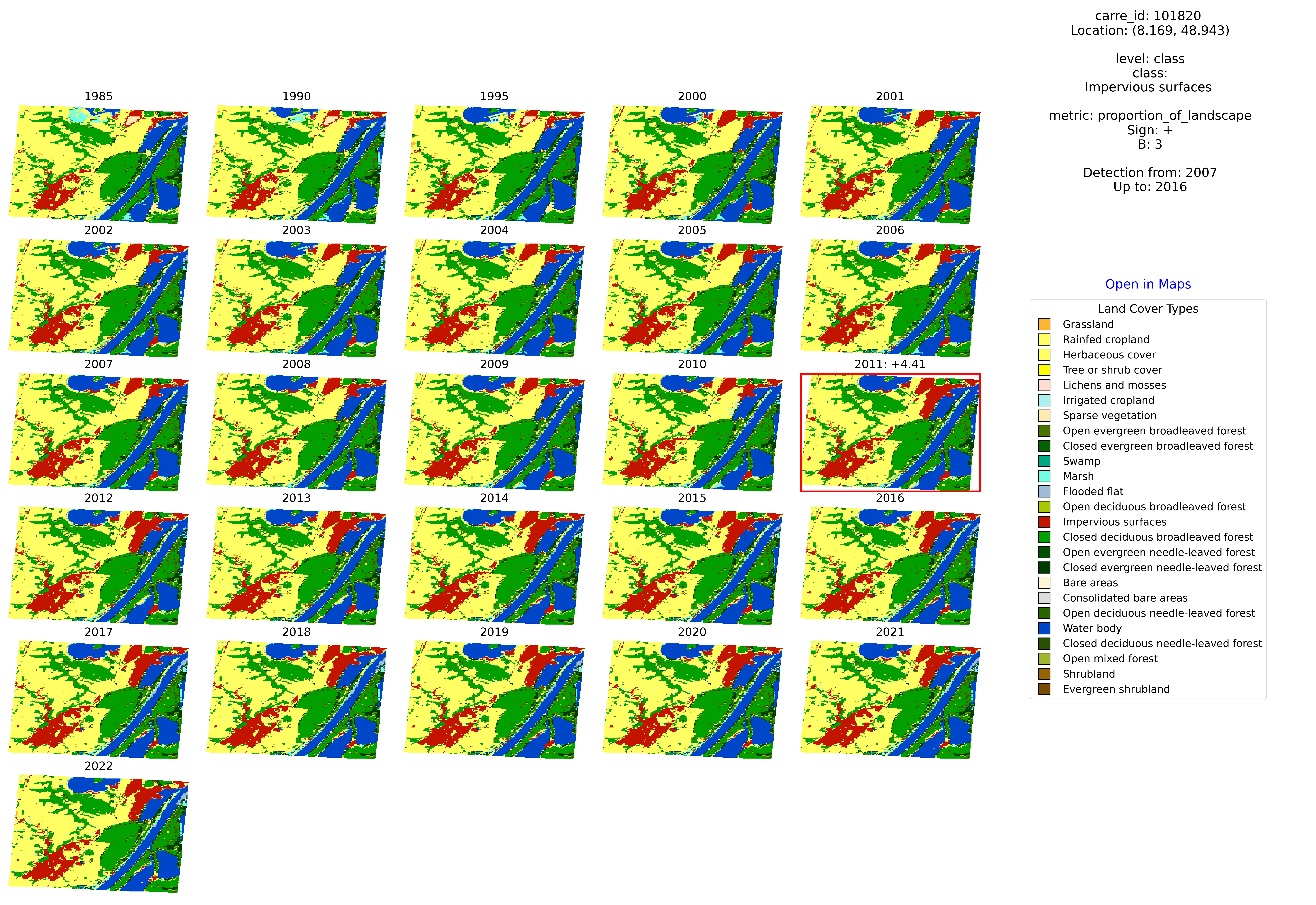
Example of detected abrupt change

 

Figure 13: Example 1 of detected abrupt change | class: Impervious surfaces, metric: proportion_of_landscape, Sign:+, B=3. Open in maps. Solar panel site construction

 

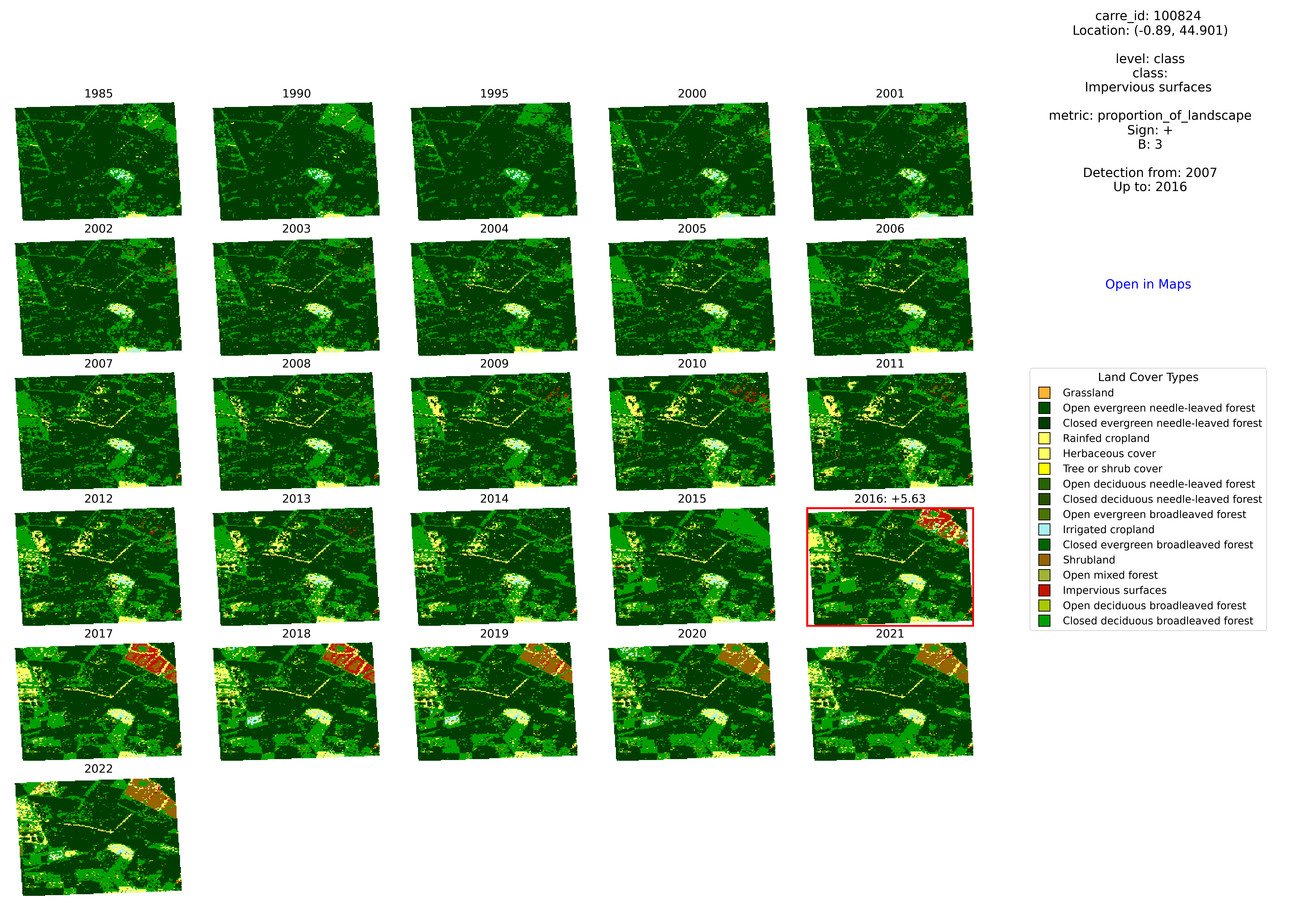
More examples

 

Figure 14: Example 2 of detected abrupt change | class: Impervious surfaces, metric: proportion_of_landscape, Sign:+, B=3. Open in maps. Boat terminal construction

 

Figure 15: Example 3 of detected abrupt change | class: Impervious surfaces, metric: proportion_of_landscape, Sign:+, B=3. Open in maps. Railroad construction

Detection events aligned on bird abundance curves

Once abrupt land cover changes detected, we can align them on the bird abundance curves as introduced before. See for instance the abundance curve of Picus viridis from Fig. 3 but with the years detected as following abrupt class propotion increase of impervious surfaces:

Figure 16: Picus viridis abundance for a selection of observation squares with detected events overlaid: abrupt class proportion increase of impervious surfaces.

Bird diversity metric shifts attribution

The objective is now to determine whether detected changes in land cover affect bird biodiversity metrics, and if so, to quantify the impact. To help us choose an appropriate method, we will use the NaviDAM filtering tool again, but this time for a different objective: Effect estimation.

NaviDAM for attribution

As we did with the Detection objective, we will now go through the different criteria options of the User input invite for the Effect estimation objective and explain them when needed.

 

Figure 17: Attribution user input | Objective, outcome and data.

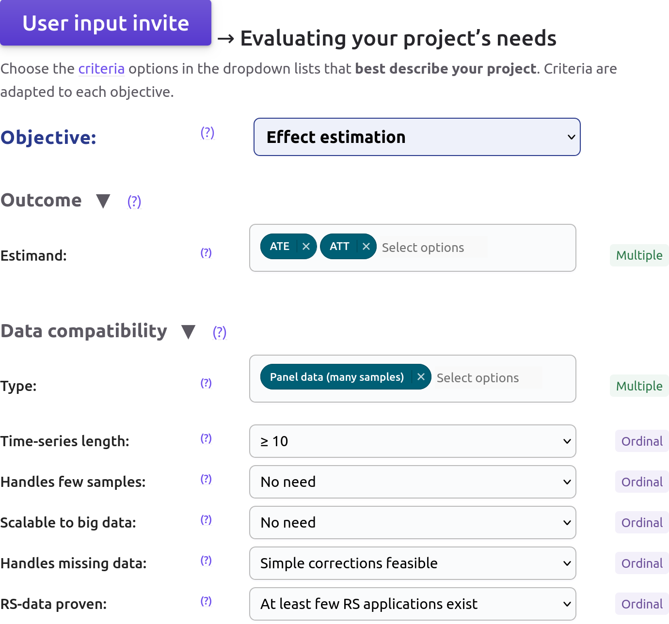
• With this second objective to attribute & quantify the effect of landscape changes, we now specify:
  • Estimand: ATE, ATT as we are interested in general effects not local or conditional ones, nor in the other suggestions.
• About the criteria on data compatibility, the requirements are the same as for the Detection objective above, details are also collapsed here:

Data compatibility details.

• Type: We have Panel data, i.e. time-series for different samples (here the STOC observation squares).
• Time-series length: We have 26 time steps, so ≥ 10 and < 100.
• Handles few samples: No need, we have thousands of points.
• Scalable to big data: No need idem. Even if we scale up the study to other monitoring programs, the relative scarcity of standardized data doesn’t require big data approaches.
• Handles missing data: Simple corrections feasible even if we have complete time-series here, we prefer imposing this condition in case remote sensing data would be missing when upscaling the study.
• RS-data proven: At least few RS applications exist no special need to rely on a estbalished method with RS data (land cover here), few applications would be enough.

 

Figure 18: Attribution user input | Model properties.

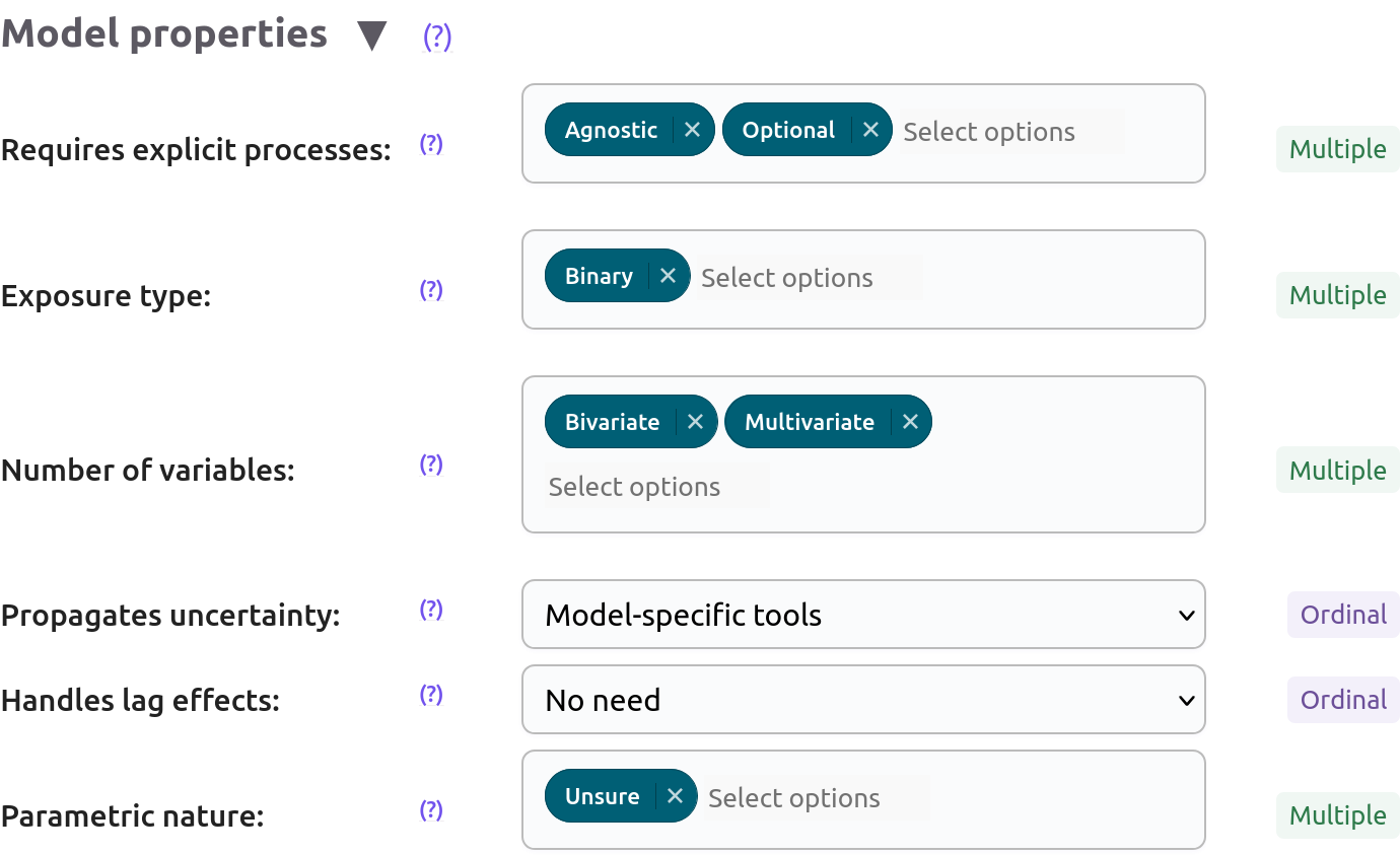
• Next come the desired model properties:
  • Requires explicit processes: Agnostic, Optional since we don’t know how to model such process here
  • Exposure type: Binary as the before/after detected abrupt change from one year to the other
  • Number of variables: Bivariate, Multivariate Here we have at least two variables in the exposure and the tested biodiversity metrics. We can even consider more than two variables at a time, e.g. to make sure to isolate the impact of landscape changes and not bioclimatic variations.
  • Propagates uncertainty: Model-specific tools - We would like at least model-specific tools (or even inherent-capacity to deal with uncertainty as it is an ordinal criteria).
  • Handles lag effects: No need because we are interested here in immediate effects of land cover change
  • Parametric nature: Unsure - Any option would actually suits us, we have no expectation so Unsure allows overpassing this criterion while indicating it as been evaluated. Letting Any would lead to same result (but an uncomplete assessment flagged), just as selecting the four non-default options.

 

Figure 19: Attribution user input | Packages.

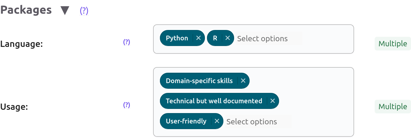
• About the expectations on packages:
  • Language: Python, R, same as for detection
  • Usage: Domain-specific skills added to User-friendly and Technical but well documented to keep maximum suggested methods and assuming the user is used to such impact analysis

 

Investigators are invited to specify method assumptions at the end of the filtering process. This way, when assumptions are not (fully) specified with Any or Unsure options, NaviDAM suggests a set of methods relying on different assumptions. This enables users to compare results across methods, assess the robustness or sensitivity of findings to assumptions, and interpret their results with multiple lines of evidence.

Figure 20: Attribution user input | Assumptions.

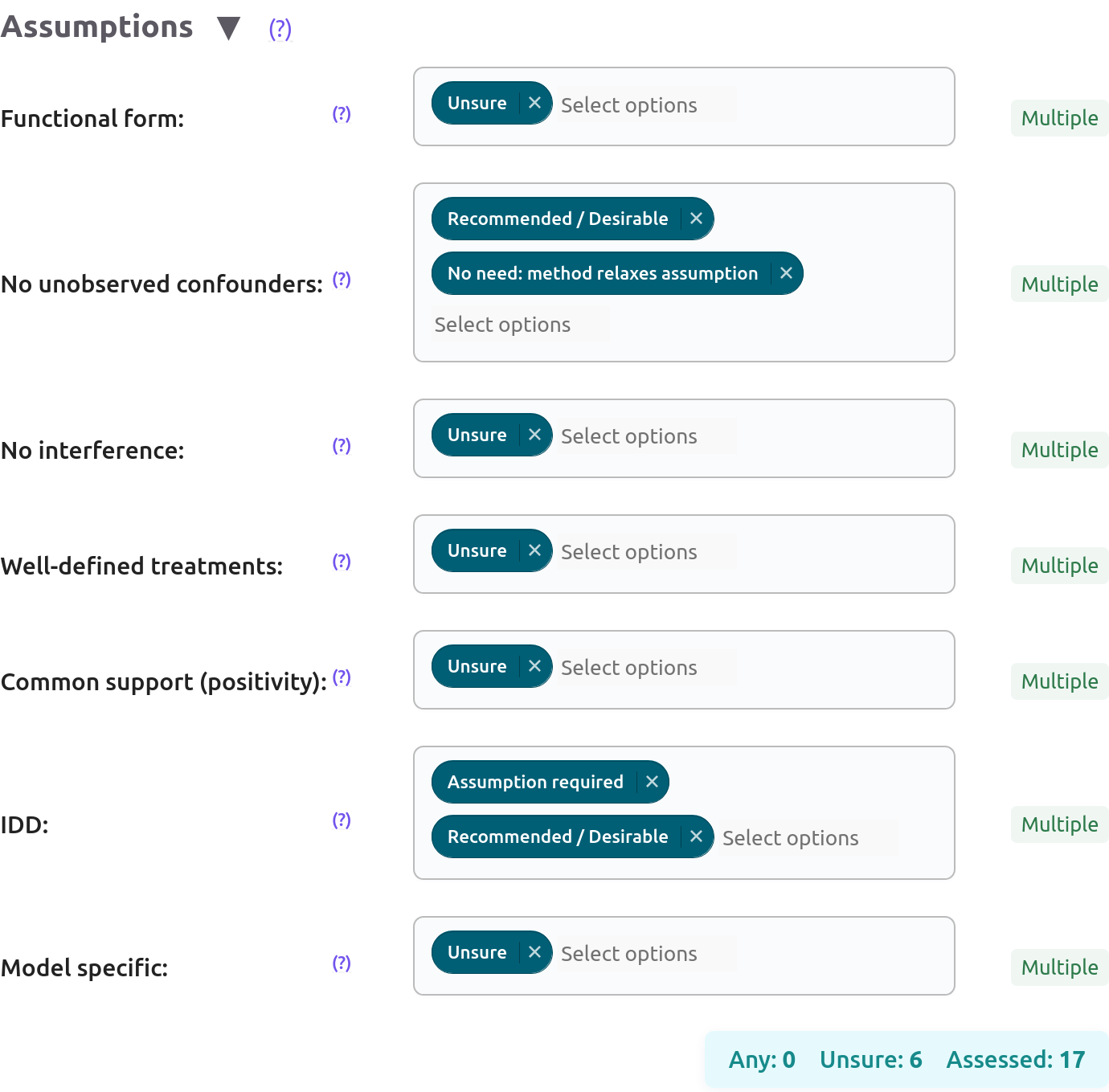
• Finally, the assumptions:
  • As indicated in the above box, a number of criteria are only informed with Unsure: It avoids filtering based on their options when the user does not want to emphasise an assumption. The opposite would be looking for a method that explicitly relaxes or firmly requires an assumption. Criteria with Unsure are note detailed here.
  • No unobserved confounders: Recommended / Desirable, No need: method relaxes assumption. In our case study, we certainly have unobserved confounders impacting both the tested outcome and our exposure. We also have observed confounders like climatic variables that will be controlled for, but others are unobserved, e.g. land use intensity. We therefore need a method that can deal with such bias, hence the chosen options.
  • IDD: Assumption required, Recommended / Desirable - We can reasonably assume having IDD samples regarding the semi-standardized sampling protocol.

--> All criteria have been assessed or at least considered with `Unsure`, so the counter on the right turns to teal.

 

Figure 21: Attribution user input | Result.

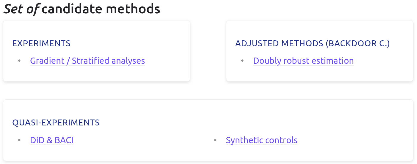
Result

A set of candidate methods belonging to three different families is suggested. As for Detection, lots of methods have still to be assessed in order to be included in NaviDAM filtering tool and we invite interested users to look at the contributing page or contact.

Since Experiments are impossible in this project, we can choose between the remaining adjusted and quasi-experimental method suggestions. We choose synthetic controls and can now consult the associated documentation page before applying them in next section.

Hands-on synthetic controls

• According to the synthetic control methodology, we gathered and aligned covariate data (bioclimatic variables, PatriNat anthropogenic pressures) on our treated sites and donor pools to then best identify suited control observation squares.
• We also computed several bird community metrics (Alpha, Beta (turnover), Shannon diversity, Pielou index) to explore the impact of land cover changes on aggregated metrics.

Status

Several variants of synthetic controls have already been applied and results will be integrated here later.

Perspectives

We plan to further exploit (Reif et al., 2021; Santini et al., 2017) to guide tests on:

• i) which bird species and populations, monitored with
• ii) which diversity metric, are sensitive to
• iii) which landscape changes.

In this gallery example, we don’t cover the significance and robustness tests independently as it could be done in the filtering tool as the page is already large. However, synthetic controls already present model-specific inherent placebo and significance tests.

References

1. Zhang, X., Zhao, T., Xu, H., Liu, W., Wang, J., Chen, X., & Liu, L. (2024). GLC_FCS30D: The First Global 30 m Land-Cover Dynamics Monitoring Product with a Fine Classification System for the Period from 1985 to 2022 Generated Using Dense-Time-Series Landsat Imagery and the Continuous Change-Detection Method. Earth System Science Data, 16, 1353–1381. https://doi.org/10.5194/essd-16-1353-2024
2. Liu, L., Zhang, X., & Zhao, T. (2023). GLC_FCS30D: The First Global 30-m Land-Cover Dynamic Monitoring Product with Fine Classification System from 1985 to 2022. Zenodo. https://doi.org/10.5281/zenodo.8239305
3. Bosch, M. (2019). PyLandStats: An Open-Source Pythonic Library to Compute Landscape Metrics. PLOS ONE, 14, e0225734. https://doi.org/10.1371/journal.pone.0225734
4. Reif, J., Szarvas, F., & Šťastný, K. (2021). ‘Tell Me Where the Birds Have Gone’ – Reconstructing Historical Influence of Major Environmental Drivers on Bird Populations from Memories of Ornithologists of an Older Generation. Ecological Indicators, 129, 107909. https://doi.org/10.1016/j.ecolind.2021.107909
5. Santini, L., Belmaker, J., Costello, M. J., Pereira, H. M., Rossberg, A. G., Schipper, A. M., Ceau\textcommabelow su, S., Dornelas, M., Hilbers, J. P., Hortal, J., Huijbregts, M. A. J., Navarro, L. M., Schiffers, K. H., Visconti, P., & Rondinini, C. (2017). Assessing the Suitability of Diversity Metrics to Detect Biodiversity Change. Biological Conservation, 213, 341–350. https://doi.org/10.1016/j.biocon.2016.08.024